43 pivot table row labels format

Overwrite pivot table conditional format based on row label As far as I know, using the one rule in the Conditional formatting, we can only format the cells with one color if the condition is true and if the same condition is false, the formatting of the cell will be blank and if both conditions are true, the formatting of cell depends on the highest ranking/priority of the rules in Conditional formatting. Formatting Pivot Table Row Labels by Level | MrExcel Message Board hover your cursor over the top line of one of the SubTotals of the Level that you want to format until you get a downward pointing, then left click - that should highlight all the cells at that level right click while hovering over one of the selected cells to format it OR hit Ctrl+F1

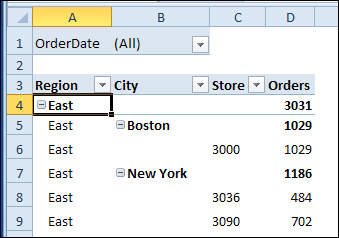
How to Change Date Format in Pivot Table in Excel - ExcelDemy Firstly, click on the Group Selection option in the PivotTable Analyze tab while keeping the cursor over a cell of the Order Date (Row Labels). Secondly, you'll get the following dialog box namely Grouping. And choose Years from the options. Finally, you'll get the sum of sales based on the years instead of the dates. 3.2.

Pivot table row labels format

Excel Pivot Table Report - Clear All, Remove Filters, Select … Pivot Table Options tab - Actions group Customizing a Pivot Table report: When you insert a Pivot Table, a blank Pivot Table report is created in the specified location, and the 'PivotTable Field List' Pane also appears which allows you to Add or Remove Fields, Move Fields to different Areas and to set Field Settings. The 'Options' and 'Design' tabs (under the 'PivotTable Tools' … Conditional Formatting in Pivot Table - WallStreetMojo Currently, a pivot table is blank. Next, we need to bring in the values. Then, drag down the "Date" in the "Rows" Label, "Name" in the "Column," and "Sales" in "Values." As a result, the pivot table will look like the one below. To apply conditional formatting in the pivot table, first, we must select the column to format. Formatting Tips for Pivot Tables - Goodly Well the filter buttons are missing from the pivots. Here are 2 ways to get it. Method 1 : Is by choosing value filters in the filter drop down of the row labels. Method 2 : Selecting the adjacent cell outside the pivot and press CTRL SHIFT L. This will directly give you a filter on the Sales Values.

Pivot table row labels format. How to Format Excel Pivot Table - Contextures Excel Tips Select a cell in any pivot table. On the Ribbon, under the PivotTable Tools tab, click the Design tab. In the PivotTable Style options gallery, right-click on the style that you want to set as the default. In the context menu, click on Set As Default. NOTE: The default PivotTable style selection is for the active workbook only. changing Date format in a pivot table - Microsoft Tech Community 4.3.2019 · @Jan Karel PieterseI have a pivot table and chart in (current) Office 365 with dates in the row column; when I follow the same steps as described below, there is no "Number Format" button showing in the Field Settings dialog - see screen copy below.Why is that? I managed to change the date format within the pivot table (using "ungroup"), but this new format does not … How to make row labels on same line in pivot table? - ExtendOffice Make row labels on same line with PivotTable Options You can also go to the PivotTable Options dialog box to set an option to finish this operation. 1. Click any one cell in the pivot table, and right click to choose PivotTable Options, see screenshot: 2. Format Pivot Table Labels Based on Date Range In the pivot table, remove any filters that have been applied - all the rows need to be visible before you apply the conditional formatting. Select all the dates in the Row Labels that you want to format. On the Ribbon, click the Home tab, and then in the Styles group, click Conditional Formatting.

Repeat item labels in a PivotTable - support.microsoft.com Right-click the row or column label you want to repeat, and click Field Settings. Click the Layout & Print tab, and check the Repeat item labels box. Make sure Show item labels in tabular form is selected. Notes: When you edit any of the repeated labels, the changes you make are applied to all other cells with the same label. How to Format Excel Pivot Table - Contextures Excel Tips 22.6.2022 · Video: Change Pivot Table Labels. Watch this short video tutorial to see how to make these changes to the pivot table headings and labels. Get the Sample File. No Macros: To experiment with pivot table styles and formatting, download the sample file. The zipped file is in xlsx format, and and does NOT contain any macros. How to Insert a Blank Row in Excel Pivot Table | MyExcelOnline 17.1.2021 · Pivot Table reports are shown in a Compact Layout format as a default and if you have two or more Items in the Row Labels (e.g.Month & Customer), then the Pivot Table report can look very clunky…. There is a cool little trick that most Excel users do not know about that adds a blank row after each item, making the Pivot Table report look more appealing. Excel Pivot Table Row Label Column Display Format Hi, I am bringing data to PivotTable from teradata database by .odc connection. Schema from which it is building dimensions, measures are created in third party tool. Now, I have a column whose datatype in database is integer, it is created as an hierarchy level, which can be brought as row ... · Right click on the cell with the number 200911, choose ...

How to Customize Your Excel Pivot Chart Data Labels - dummies Excel displays the Format Data Labels pane. Check the box that corresponds to the bit of pivot table or Excel table information that you want to use as the label. For example, if you want to label data markers with a pivot table chart using data series names, select the Series Name check box. How to Use Excel Pivot Table Label Filters - Contextures Excel Tips To change the Pivot Table option, and allow multiple filters, follow these steps: Right-click a cell in the pivot table, and click PivotTable Options. In the PivotTable Options dialog box, click the Totals & Filters tab. In the Filters section, add a check mark to 'Allow multiple filters per field.'. Click the OK button, to apply the setting ... Automate Pivot Table with Python (Create, Filter and Extract) 22.5.2021 · Photo by Jasmine Huang on Unsplash. In Automate Excel with Python, the concepts of the Excel Object Model which contain Objects, Properties, Methods and Events are shared.The tricks to access the Objects, Properties, and Methods in Excel with Python pywin32 library are also explained with examples.. Now, let us leverage the automation of Excel report with Pivot … Change Pivot Table Layout using VBA - Access-Excel.Tips You can change any label in the Pivot Table. To change RowLabels and Column Labels ActiveSheet.PivotTables ("PivotTable1").CompactLayoutRowHeader = " NewRowName " ActiveSheet.PivotTables ("PivotTable1").CompactLayoutColumnHeader = " NewColumnName " To change "Grand Total" ActiveSheet.PivotTables ("PivotTable1").GrandTotalName = " NewGrandTotal "

Excel compare list

Excel Pivot Table - Format Numbers in Rows To format rows or columns in a PT, hover the mouse at the top of the column or beginning of the row until a black arrow appears, click to highlight the row/column and format as usual. For Display labels from next field in same column, uncheck this, follow above procedure, then recheck. Paula Scharf

Excel 2010 - Pivot Table - How to print repeating row labels at the top of every new page

How to rename group or row labels in Excel PivotTable? - ExtendOffice To rename Row Labels, you need to go to the Active Field textbox. 1. Click at the PivotTable, then click Analyze tab and go to the Active Field textbox. 2. Now in the Active Field textbox, the active field name is displayed, you can change it in the textbox.

Repeat Pivot Table Labels in Excel 2010 - Excel Pivot TablesExcel Pivot Tables

Design the layout and format of a PivotTable To change the format of the PivotTable, you can apply a predefined style, banded rows, and conditional formatting. Windows Web Mac Changing the layout form of a PivotTable Change a PivotTable to compact, outline, or tabular form Change the way item labels are displayed in a layout form Change the field arrangement in a PivotTable

How to make row labels on same line in pivot table?

How to Create a Pivot Table in Excel: A Step-by-Step Tutorial 31.12.2021 · Highlight your cells to create your pivot table. Drag and drop a field into the "Row Labels" area. Drag and drop a field into the "Values" area. Fine-tune your calculations. Now that you have a better sense of what pivot tables can be used for, let's get into the nitty-gritty of how to actually create one. Step 1.

Sort multiple row label in pivot table - Microsoft Community

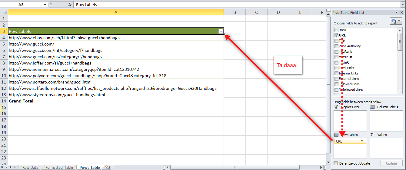
Pivot Table "Row Labels" Header Frustration Pivot Table "Row Labels" Header Frustration. Hi Everyone please help I can't change my headers from Row Labels in a Pivot Table. Using Excel 365. Labels:

SQL Server Data Analysis and Reporting Tools

Quick tip: Rename headers in pivot table so they are presentable 15.3.2018 · Pivot tables are fun, easy and super useful. Except, they can be ugly when it comes to presentation. Here is a quick way to make a pivot look more like a report. Just type over the headers / total fields to make them user friendly. See this quick demo to understand what I mean: So simple and effective.

Pivot table row labels in separate columns • AuditExcel.co.za

How to Add Rows to a Pivot Table: 9 Steps (with Pictures) 10.8.2022 · Reorder the field labels in the "Row Labels" section. If you already have a field in the Rows area, adding another row below that will nest the new row within the existing row. [2] X Trustworthy Source Microsoft Support Technical support and product information from Microsoft.

Pivot Table Multiple Row Labels Side By Side | Decorations I Can Make

Pivot table row labels side by side - Excel Tutorials - OfficeTuts Excel You can copy the following table and paste it into your worksheet as Match Destination Formatting. Now, let's create a pivot table ( Insert >> Tables >> Pivot Table) and check all the values in Pivot Table Fields. Fields should look like this. Right-click inside a pivot table and choose PivotTable Options…. Check data as shown on the image below.

Repeat all labels in an Excel pivot table | The Right Join

PDF Excel Troubleshooting Row Labels in Pivot Tables In Excel 2007 and earlier, you had to follow these steps: 1. Select the entire pivot table. 2. Copy the pivot table to the clipboard. 3. Use the Paste Special dialog to paste just the Values. This will change the report from a live pivot table to a static report. 4. Select the first blank column cell to the last blank column cell. 5.

Centre Column Headings in Excel Pivot Table – Excel Pivot Tables

PowerPivot row labels - Microsoft Tech Community In Power Pivot there are no row headers, that's only columns headers. If you try to rename it in Power Pivot it'll be a message. thus it's hard to rename them eventually. And after the refresh column names in Power Pivot are returned back. If you renamed row labels in PivotTable they are not synced back to the source.

How to Create a MS Excel Pivot Table – An Introduction | SIMPLE TAX INDIA

Pivot Table Row Labels In the Same Line - Beat Excel! Learn how to arrange pivot table roow labels in the same line. Put multiple lables side by side into the same line. ... It is a common issue for users to place multiple pivot table row labels in the same line. ... bar chart Basics column chart Combined Charts comment condition conditional formatting data analysis data validation data ...

How to Sort Pivot Table Row Labels, Column Field Labels and Data Values with Excel VBA Macro ...

How to Apply Conditional Formatting to Pivot Tables Select a cell in the Values area. The first step is to select a cell in the Values area of the pivot table. If your pivot table has multiple fields in the Values area, select a cell for the field you want to apply the formatting to. 2. Apply Conditional Formatting. You can find the Conditional Formatting menu on the Home tab of the Ribbon.

Repeat Pivot Table row labels • AuditExcel.co.za Pivot Tables Course

Automatic Row And Column Pivot Table Labels - How To Excel At Excel Select the data set you want to use for your table The first thing to do is put your cursor somewhere in your data list Select the Insert Tab Hit Pivot Table icon Next select Pivot Table option Select a table or range option Select to put your Table on a New Worksheet or on the current one, for this tutorial select the first option Click Ok

Create Multiple Subtotals in a Pivot Table – Excel Pivot Tables

How to Create Excel Pivot Table (Includes practice file) 28.6.2022 · What’s an Excel Pivot Table? You might think of a pivot table as a custom-created summary table of your spreadsheet. It’s a little bit like transpose in Excel, where you can switch your columns and rows.But it also has elements of Excel Tables.And like tables, you can use Excel Slicers to drill down into your data.. You create the pivot table by defining which fields to …

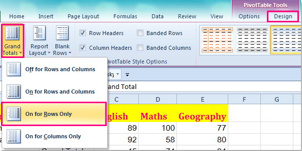
How to display grand total at top in pivot table?

Change Blank Labels in a Pivot Table - Contextures Blog In a pivot table, you might have a few row labels or column labels that contain the text "(blank)". This happens if data is missing in the source data. For example, in the source data, there might be a few sales orders that don't have a Store number entered. ... copy the formatting from one pivot table, and apply it to another pivot table ...

Pivot Tables Excel 2007 Row Labels Side By | Brokeasshome.com

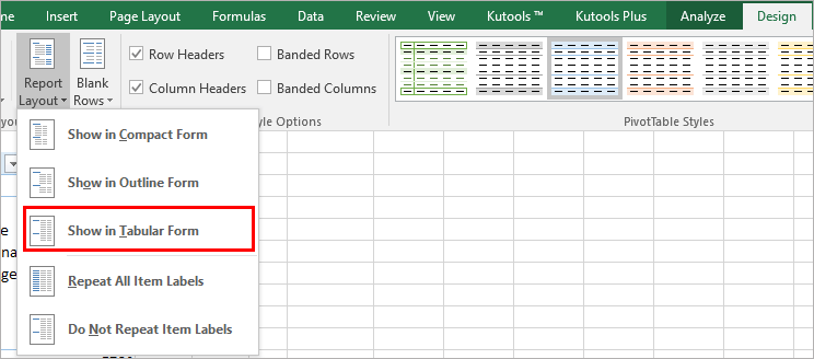
Remove row labels from pivot table • AuditExcel.co.za Click on the Pivot table. Click on the Design tab. Click on the report layout button. Choose either the Outline Format or the Tabular format. If you like the Compact Form but want to remove 'row labels' from the Pivot Table you can also achieve it by. Clicking on the Pivot Table. Clicking on the Analyse tab.

Excel pivot table – How it works

Pivot table row labels in separate columns • AuditExcel.co.za Our preference is rather that the pivot tables are shown in tabular form (all columns separated and next to each other). You can do this by changing the report format. So when you click in the Pivot Table and click on the DESIGN tab one of the options is the Report Layout. Click on this and change it to Tabular form.

Share :